This post is based on “Tenzorized Embedding Layers” paper. Here, I’d like to explain the main ideas from this paper and show some results.

One of the key components of natural language processing (NLP) models is embedding layers, which transform input words into real vectors. This can be represented as a lookup table (or a matrix). The large vocabulary leads to enormous weight matrices. State-of-the-art NLP networks are large, with millions to billions of parameters. However, computational resources are oftern limited, which is an essential problem in NLP research. What can we do about that?

The purpose of tensor decompositions is to represent a given tensor as a product of smaller tensors called cores with fewer parameters while preserving important information.

Tensor decompositions, such as Tucker decomposition, canonical decomposition, and Tensor Train (TT) decomposition (1), can be applied for dimensionality reduction in a varity of tasks. For instance, signal and data compression, or compression of neural networks layers. In the last case, model parameters are factorized into smaller cores of the corresponding tensor decomposition. For example, TT decomposition was utilized for a compression of a linear layer (2), what was extended to a compression of convolutional layer with canonical decomposition (3). The same holds for Tensor Ring (TR) decomposition (4).

Here, I’d like to show how TT and TR decompositions can be used to compress the embedding layer. $\def\uuX{\underline{\bf X}}$ $\def\uuG{\underline{\bf G}}$ $\newcommand\R{\mathbb{R}}$ $\newcommand\bG{\bf G}$ $\newcommand\bX{\bf X}$ $\newcommand\bU{\bf U}$ $\newcommand\bV{\bf V}$

Tensor Train decomposition

Suppose we have a $N$th-order tensor $\uuX \in \R^{I_1 \times I_2 \times \dots \times I_N}$. The TT representation of $\uuX$ is given as

or, equivalently,

where slice matrices are defined as \({\bG}_{i_n}^{(n)} =\) $\uuG^{(n)}(:, i_n, :) \in \mathbb{R}^{R_{n-1} \times R_n}, i_n = 1, 2, \dots, I_N$ with $\uuG^{(n)}$ being the $i_n$th lateral slice of A core tensor $\uuG^{(n)} \in \mathbb{R}^{R_{n-1}\times I_n \times R_n},$ $n=1, 2, \dots,N$ and $R_0 = R_N = 1$ by definition.

The key idea of TT decomposition is demonstrated in the next figure. The minimal values of ${R_k}_{k=1}^{N-1}$ are called TT–ranks for which the TT–decomposition exists.

The total number of parameters in TT decomposition can be evaluated as $\sum_{k=1}^N R_{k-1} I_k R_{k}$. Hence, if there are core tensors with small ranks, the total number of elements required to represent a given tensor in TT–format is significantly smaller than the number of elements in a full tensor $\sum_{k=1}^N I_k$. This remark makes the application of TT decomposition appealing in a lot of problems related to extremely large data.

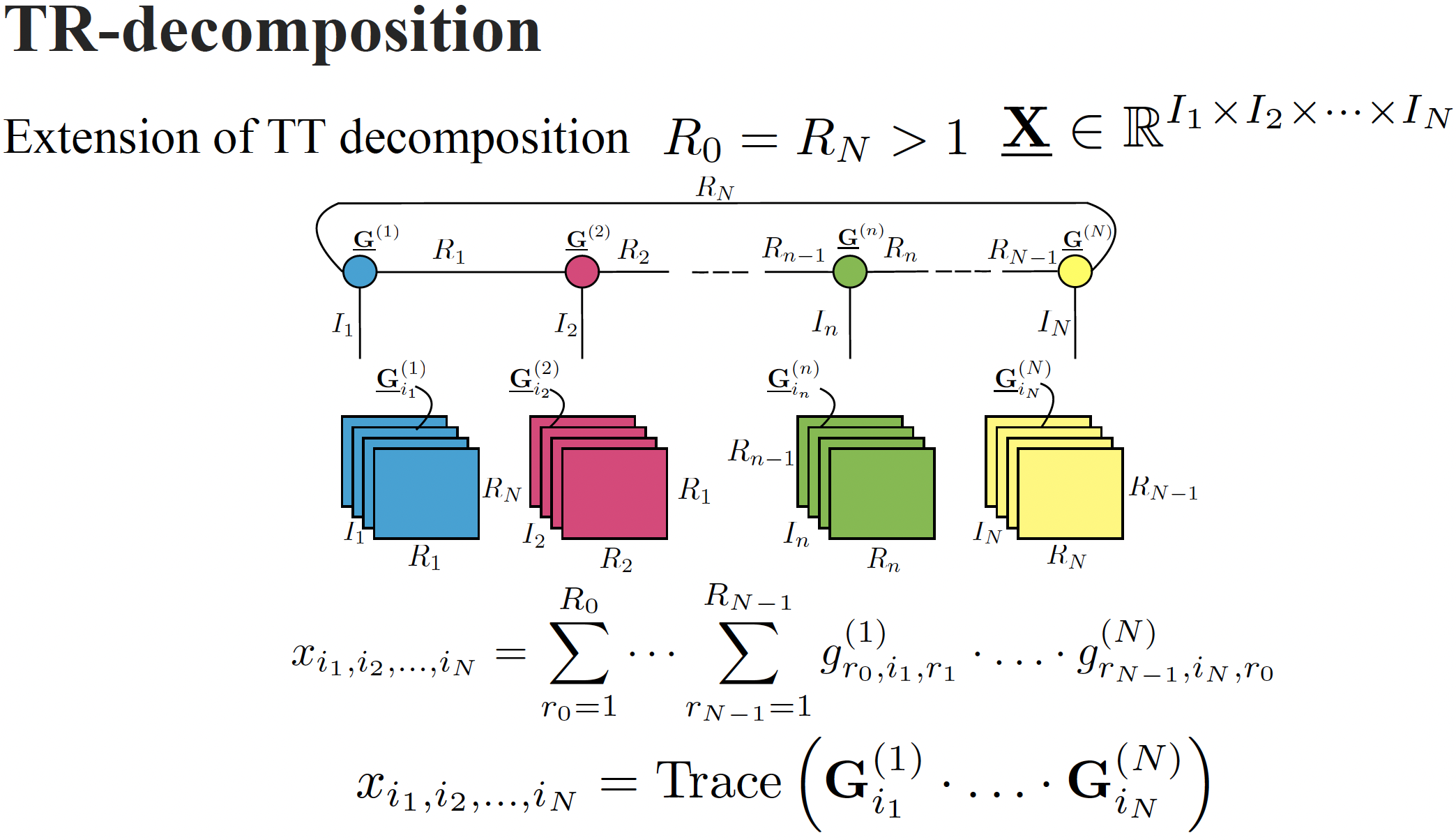
Tensor Ring decomposition

The tensor ring format of a tensor $\uuX \in \mathbb{R}^{I_1 \times \cdots \times I_N}$ is defined as

or in index-form

where \({\bG}^{(n)}_{i_n}\) is an $i_n$th slice matrix of a tensor $\uuG^{(n)}$ $\in \R^{R_{n-1}\times I_n \times R_n}$. The last latent tensor $\uuG^{(N)}$ is of size $R_{N-1} \times I_N \times R_0$, i.e., $R_{N} = R_0$.

The TR-format can be seen as a natural extension of the TT decomposition where $R_0=R_N=1$. The illustration of TR-format is given in next figure.

However, the TR-format is known to have theoretical drawbacks compared to TT decomposition (5). For example, it was found that in case of TR decomposition, minimal TR-ranks for a tensor need not be unique (6) (not even up to permutation of the indices $i_1, \dots , i_N$), resulting in problems in their estimation. On the other hand, numerical experiments show that the TR-format leads to lower ranks of the core tensors compared to the TT-format (7), which means higher compression ratios and lower storage costs.

TT and TR embeddings

We aim to replace a regular embedding matrix with a more compact, yet powerful and trainable, format which would allow us to efficiently transform input words into vector representations.

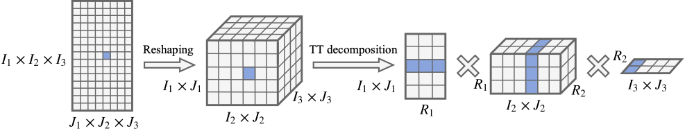
Let $\bX \in \mathbb{R}^{I \times J}$ be a matrix of size $I \times J$. The goal is to get natural factors of its dimensions $I = \prod_{n=1}^N I_n$ and $J = \prod_{n=1}^N J_n$ and then reshape this matrix to $N$th-order tensor $\uuX \in \mathbb{R}^{I_1 J_1 \times I_2 J_2 \times \dots \times I_N J_N}$ whose $n$-th dimension is of length $I_n J_n$ and is indexed by the tuple $(i_n , j_n)$. We also can treat this procedure as the bijection that map rows and columns of the original matrix to the $N$-dimensional vector-indices. Than TT decomposition according to Eq. (1) is applied to this tensor to get a compact representation:

The described representation of a matrix in the TT–format is called a TT–matrix. The obtained factorizations $(I_1, I_2, \dots I_N ) \times (J_1,J_2, \dots J_N)$ will be treated as shapes of a TT– matrix, or TT–shapes. The idea of constructing the TT– matrix from a given matrix is showed in next figure for a 3-dimensional tensor.

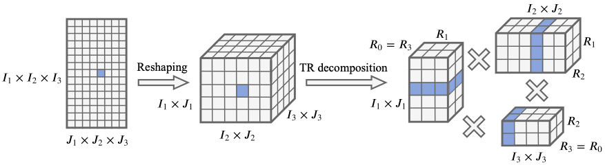
Similarly, we can define a TR-matrix by reshaping a given matrix $\bX$ into a tensor $\uuX \in \mathbb{R}^{I_1 J_1 \times I_2 J_2 \times \dots \times I_N J_N}$:

A concept of building the TR– matrix from the given matrix is showed in next figure for a 3-dimensional tensor.

Now we can introduce a concept of a tensorized embedding layer:

A TT/TR-embedding layer is a layer where TT/TR–cores are trainable parameters, and they are represented as a TT/TR–matrix which can be transformed into an embedding layer $\bX \in \mathbb{R}^{I \times J}$. The algorithm requires to set the ranks in advance to define the cores size, and they are considered to be hyperparameters of the layer. The ranks values are crucially important since they determine and control the compression ratio.

To obtain an embedding for a specific word indexed $i$ in a vocabulary, we transform a row index $i$ into an N-dimensional vector index $(i_1; : : : ; i_N)$, and compute components of TT or TR embedding. Note, that the evaluation of all its components is equal to choosing the specific slices and running a sequence of matrix multiplications, which is implemented efficiently in modern linear algebra modules.

Results

Let me show results on a simple task – sentiment analysis. Sentiment analysis refers to predicting a polarity of a sentence.

The proposed approach is compared with the following baselines:

• Standard embedding layer with the baseline compression ratio 1.
• Embedding layer is parametrized by two matrices $\bX = \bU \bV^T$ where $\bU \in \R^{I\times R}$ and $\bU \in \R^{J\times R}$. Then the compression ratio is $\frac{IJ} {(I+J)R} \sim \frac{J}{R}$.

We test our approach on popular datasets such as the IMDB dataset with two classes, and the Stanford Sentiment Treebank (SST) with five classes. Our model consists of a standard bidirectional two-layer LSTM with a hidden size of 128 and a dropout rate of 0.5. For the embedding layer, we used the most frequent 25,000 words for IMDB and 17,200 for SST, and transformed them into a J-dimensional space with a regular embedding layer or a TT/TR embedding layer.

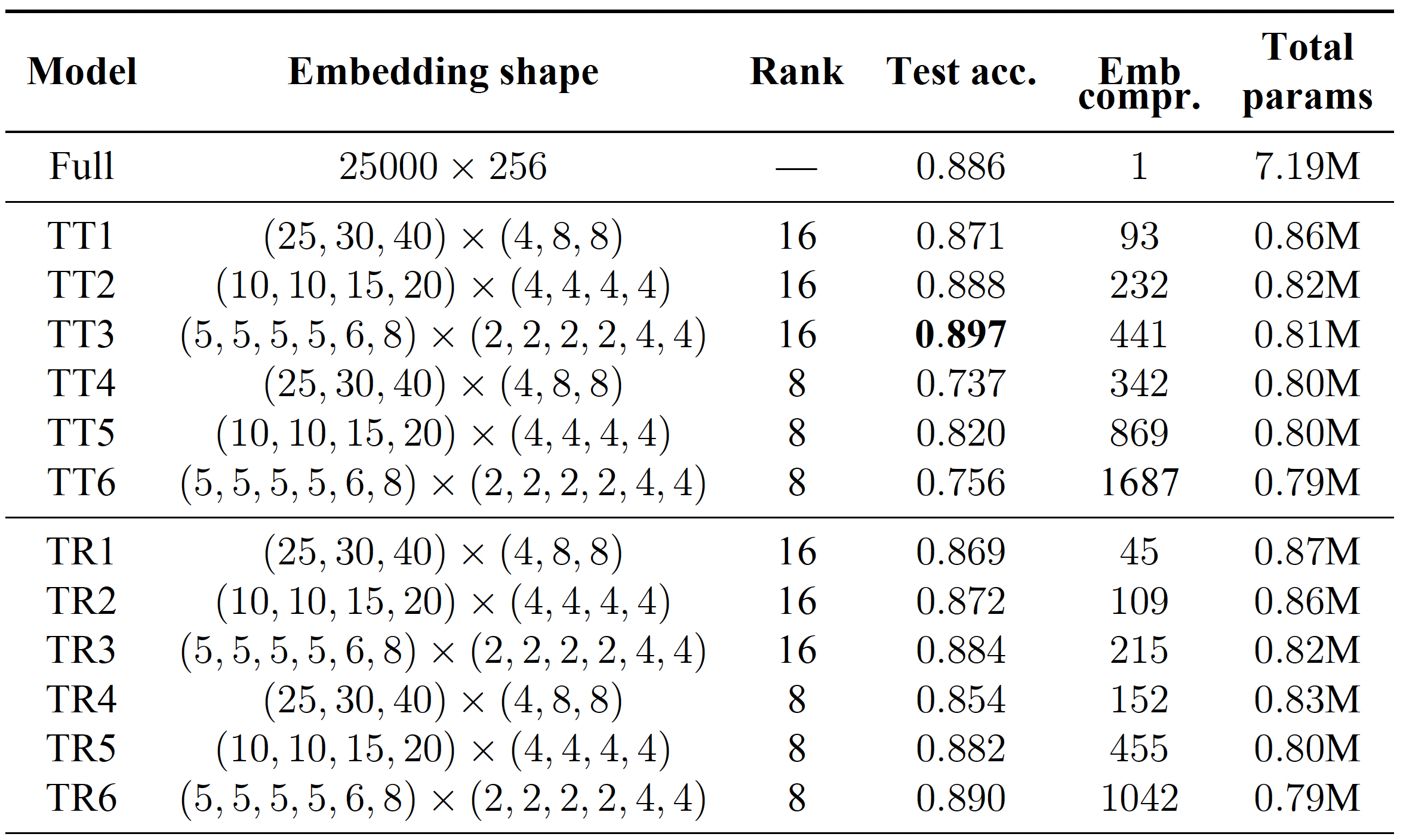
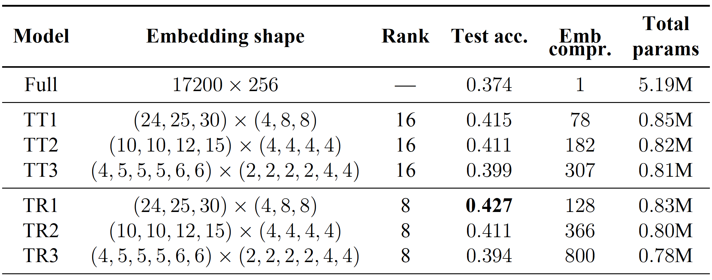
The results of our experiments reveal that the models with the compressed embedding layer performed similarly or even better than the models with standard embedding layers. For example, on the IMDB dataset, the TT embedding layer with a rank of 16 and a test accuracy of 89.7% outperformed our baseline model with a test accuracy of 88.6%. Furthermore, the compressed model had significantly fewer parameters than the full model (7.19 million vs less than a million). Similarly, on the SST dataset, the model with the TR-embedding layer outperformed both the model with the regular embedding layer and the TT layer. In the case of matrix low-rank factorization, we would obtain compression ratios $\frac{J}{R} = \frac{256}{8} =32$ or $\frac{256}{16}= 16$ which are definitely worse compared to tensor factorization techniques.

The obtained slightly better test accuracy of the models with tenzorized embedding layers suggests that imposing specific tensorial low–rank structure on the matrix of embedding layer can be considered as a particular case of regularization, thus, potentially the model generalize better.

Conclusion

To conclude, TT and TR decompositions can be used to compress neural networks. We use them to compress embedding layers in NLP models. This method can be easily integrated into any deep learning framework and trained via backpropagation, while capitalizing on reduced memory requirements and increased training batch size. More details can be found in the paper and code is available here.

References

1. Oseledets, Ivan V. “Tensor-train decomposition.” SIAM Journal on Scientific Computing 33.5 (2011): 2295-2317.
2. Novikov, Alexander, et al. “Tensorizing neural networks.” Advances in neural information processing systems 28 (2015).
3. Lebedev, Vadim, et al. “Speeding-up convolutional neural networks using fine-tuned cp-decomposition.” arXiv preprint arXiv:1412.6553 (2014).
4. Wang, Wenqi, et al. “Wide compression: Tensor ring nets.” Proceedings of the IEEE Conference on Computer Vision and Pattern Recognition. 2018.
5. Grasedyck, Lars, Daniel Kressner, and Christine Tobler. “A literature survey of low‐rank tensor approximation techniques.” GAMM‐Mitteilungen 36.1 (2013): 53-78.
6. Ye, Ke, and Lek-Heng Lim. “Tensor network ranks.” arXiv preprint arXiv:1801.02662 (2018).
7. Zhao, Qibin, et al. “Learning efficient tensor representations with ring-structured networks.” ICASSP 2019-2019 IEEE international conference on acoustics, speech and signal processing (ICASSP). IEEE, 2019.